Recently I created a basic Discord bot for the school’s computing club group using the Discord.js library for Node.js.
At the moment it has basic functionality such as replying to mentions with random messages, making “I’m dad” jokes and welcoming new members.
After I created the bot I thought it would be interesting to try and add a GUI to let me turn parts of it on and off. I’d never used Electron before so I thought I’d try it out.
I used Comic Sans (of course) and ended up with the following HTML and CSS interface:
I was pleasantly surprised by how easy it was to create the Electron interface. I obviously haven’t done a brilliant job of designing it, but the process of adding it to the Node.js app was simple. I’m looking forward to using Electron again in future projects.
At the moment the code is a bit of a mess because I added the Electron GUI after everything else. The code for the bot itself is located in the main process instead of the renderer process, so I have to use IPC messages for the GUI to communicate with the bot. In the future I might refactor it so that the bot runs in the renderer process instead.
While writing it I made the mistake of including the node_modules folder in the Git repository. It turns out that the Electron executable is more than 100MB, which is bigger than the maximum file size allowed on GitHub. I found a solution on Stack Overflow to remove the node_modules folder from my commits before I pushed them to GitHub, which solved the problem.
Recently I’ve been watching some of Ben Eater’s videos on Youtube about building a computer following the SAP-1 architecture. To practice using TypeScript I decided to try and create a simulator.
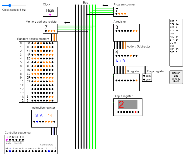
I wanted to be able to see what was going on, so I used p5.js to create a graphical interface showing the state of the different components.
You can adjust the clock speed using the slider in the top left corner, and you can write assembly programs and write them to the RAM using the textarea and button on the right.
The default program that is running when the page loads calculates the Fibonacci sequence, restarting when it goes over 255 because the computer can only store 8 bit numbers.
The computer
The computer is a simulation based on Ben Eater’s implementation of the SAP-1 (Simple As Possible 1) architecture by Albert Malvino in the book Digital Computer Electronics. (I’d like to look at the original book but am yet to find a library that has it).
I’ve simplified Ben Eater’s physical implementation slightly by having all of the control signals active high instead of a mix of active low and active high.
The architecture is made up of 11 components with 16 control signals.
Component
Description
Control signals
Clock
Alternates between high and low at a specific frequency to coordinate the timings of the computer’s activities.
halt
Memory address register
Stores the RAM address that is being read from or written to.
mar in
Random access memory
Stores 16 bytes of machine code instructions and data.
ram in, ram out
Instruction register
Stores the instruction that is currently being executed so that the controller sequencer can issue the correct control signals at a given time step.
instruction in, instruction out
Controller sequencer (or control unit)
Allows the computer to carry out instructions by issuing control signals to coordinate how the other components interact. It carries out each instruction by counting through six time steps and writing control signals using pre-programmed microcode logic that is based upon the instruction register’s contents, the time step and the flags register.
Program counter
A counter that stores which instruction should be fetched and executed next.
counter out, counter increment, jump
A register
A general purpose register that is the first input to the adder/subtractor. The ADD and SUB instructions store the result in this register.
a in, a out
Adder/ subtractor
The adder/subtractor either adds the contents of the A and B registers together or subtracts them based on the subtract control signal. It isn’t an ALU because it can’t carry out logical operations.
sum out, subtract
B register
The B register is the second input to the Adder/ subtractor. The ADD and SUB instructions store the number to be added or subtracted in this register.
b in
Output register
This register stores the output of the computer, which is shown on a display. The OUT instruction writes the contents of the A register here.
output in
Flags register
Stores the carry and zero flags from the adder/subtractor. These are used by the controller sequencer in conditional jump instructions JC and JZ.
flags in
There are 11 assembly instructions the computer can execute:
Instruction
Description
NOP
Do nothing
LDA
Load the value in the specified memory address into the A register.
ADD
Add the value in the specified memory address with the value in the A register, storing the result in the A register.
SUB
Subtract the value in the specified memory address from the value in the A register, storing the result in the A register.
STA
Store the value in the A register in the specified memory address.
LDI
Immediately load the specified value into the A register without involving memory.
JMP
Jump to the specified instruction number.
JC
Jump to the specified instruction number if the carry flag is set.
JZ
Jump to the specified instruction number if the zero flag is set.
OUT
Load the value in the A register into the output register to be shown on a display.
HLT
Stop the computer clock.
Graphics
A coloured line or circle represents a 1, and a black line or circle represents a 0.
Connections between the components and the bus are only shown when they are actively reading or writing to it. This represents the tri-state buffers, which electrically disconnect the components from the bus when the control bits dictate that they are not reading or writing.
The arrows above connections show whether the component is reading or writing. For example, in the diagram above, the program counter is writing the number 7 to the bus while the memory address register is reading and storing this value.
I implemented the graphics separately to the computer simulator itself so that the computer could still be used in other contexts without any modification. To do this I created a computerState object that tracks the state of components and calls the relevant graphics functions whenever something changes.
Implementation
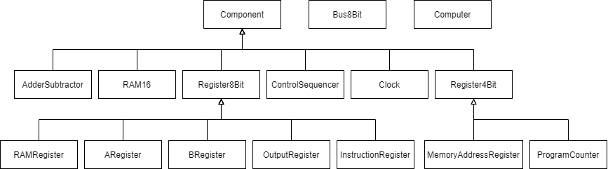
I implemented each component of the computer as a class and then created a Computer class that combined all these together to form the full computer. I used inheritance from an abstract Component class to ensure that I kept a uniform interface for all the components.
Inheritance diagram
Up until now I have created JavaScript projects by having different files and then including them all using the HTML script tags. However, this was more difficult to do with TypeScript because the transpiler would not know that the files were linked together like this and would give error messages when I tried to use variables and classes from other files.
As a result, I decided to try and implement the computer as an ES6 module with import and export statements. Although this was confusing at first and it took me a while to get it to work I have learned how to get TypeScript to transpile correctly and how to use a module, which I am happy about.
I have enjoyed watching Ben Eater’s videos and creating this simulation. It was nice to see the theory I’d done in GCSE Computer Science such as the fetch-execute cycle and components such as the program counter in action, even on such a small scale.
Recently I’ve been using the Phaser JavaScript game framework to create a game with a friend. I thought that it would be interesting to use what I’ve learned to create a basic game that a genetic algorithm can play.
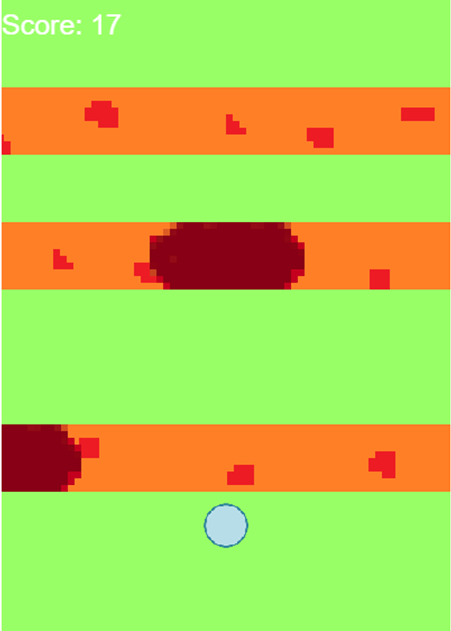
I ended up with a simple game where the player has to jump over rocks floating on lava streams using the space bar. I made the graphics myself so they are, to put it lightly, rather lacking.
You can try playing the game in your browser here, and the code is all on GitHub here.
The next step was to add a genetic algorithm. I modified the game by removing the code that let the user play and adding some methods to get data about the position of rocks and whether there is grass at a particular y coordinate.
The genetic algorithm evolves weights for a logistic regression classifier that decides whether the player should jump forward or not. I made a LogisticRegressionClassifier class as well as an Agent class that represents a single player and a GeneticAlgorithm class that manages the population of agents and carries out selection, crossover, mutation and elitism.
You can try running the genetic algorithm in your browser here and you can see the code on GitHub here.
The genetic algorithm does actually seem to learn! For example on generation 1 below it was pretty hopeless with the highest score being 7.
The agents are opaque – if they appear solid it means that there are multiple agents on top of each other (quite confusing to look at).
However, by generation 39 it has learned and some of the agents are able to get scores over 30, which is where the lava streams stop on the modified version of the game.
The lava gets faster as they go further
I wrote a more detailed walk-through of the code for creating the game on the Micropi blog here, and a walk-through of the genetic algorithm code here.
I recently finished the free online machine learning course by Stanford University professor Andrew Ng on coursera. It gives a grounding of the core concepts of machine learning such as cost functions and gradient descent and explores how different supervised and unsupervised learning algorithms such as linear regression, neural networks, support vector machines and K-means clustering work.
I was able to follow most of the maths thanks to the level 2 Further Maths course we finished before the lockdown although I did get lost in the optional modules explaining support vector machines.
I found the course extremely interesting and engaging and have learnt a lot. I followed the recommended due dates for the weekly quizzes and programming assignments to finish in 11 weeks.
I had to use Octave for the programming assignments, which is a high-level programming language designed for making numerical computations using matrices and vectors and which is mostly cross-compatible with MATLAB. It was very different to Python and JavaScript but I quite enjoyed using it once I got used to the basics. The main thing that I couldn’t get used to was indexing starting at 1 instead of 0 (the horror!).
I’m looking forward to applying my new knowledge on machine learning problems.
The 555 timer is the most popular integrated circuit ever produced – in 2003 it was estimated that a billion units are manufactured every year. It is used for many applications involving oscillating, pulse generation and timing.
Recently I was set the challenge of simulating a 555 timer circuit using JavaScript. this is what I ended up with:
On the top of the screen is a graph showing the voltage level on the output pin of the 555 IC and the voltage level on the anode of the capacitor (relative to ground).
On the left are sliders that allow you to adjust the resistances of the two resistors and the capacitance of the capacitor. There are also labels showing the duty cycle and frequency of the output square wave. Additionally, you can adjust the milliseconds per division of the graph.
On the right is a diagram of the circuit, showing all of the internal components within the IC. The wires between components change colour depending on the voltage on them (relative to ground), where green is 9v and red is 0v.
I used p5.js for the graphics because it’s extremely easy to use and is compatible with most browsers.
If you’d like to try out the simulation you can access it here: https://brychanthomas.github.io/555/. Although it seems to work on mobile devices it is better on computers with bigger screens and better processors. I found that Chrome was the best web browser for it.
Design
Instead of just using the equations that describe the behaviour of the 555 timer as a black box, I thought that I’d simulate the individual components inside the IC in order to learn more about how it works. I based my circuit upon this diagram:
As you can see, to implement this circuit I had to create objects representing resistors, comparators, SR flip-flops and transistors. I didn’t include the reset and control voltage pins because they weren’t necessary for the circuit I was planning to build, although adding them could be a future improvement.
When I first implemented this circuit the output pin was low when the capacitor was charging and high when it was discharging, when it should be the other way round. Looking at the datasheet for the NE555 I saw that there is supposed to be a NOT gate between the complement of Q on the flip flop and the output pin – I think this is represented by the ‘Output Driver’ in the above diagram. Instead of having to fit in a NOT gate I decided to just connect the output pin to the Q pin instead of the Q complement pin, as in this diagram.
Then, in order to create the circuit, I added the external components by following the below diagram:
This sets up the IC as an astable multivibrator, which means that it continually oscillates between two states where the output is either high or low. I had to simulate a capacitor to do this. I used this equation to simulate the charging of the capacitor and this equation to simulate its discharging.
I implemented each electrical component as a class in order to make it easier to re-use the code in any other projects I do. It also made it easy to have multiple instances of one type of component. As well as these classes I needed a class that handled the graph, a class that handled drawing the circuit components each frame, a class that handled drawing the coloured lines between components each frame and a class for the overall 555 timer IC that depended on the component classes.
Simplification
I stuck to simulating voltages without calculating currents. All of the equations and logic I used to simulate the components were based on voltages and, for the capacitor, time, so there was no need to calculate the current in different parts of the circuit. I stored all of the voltages in a dictionary called ‘voltages’, where each point in the circuit is stored as a key:value pair with a string key such as ‘b+’ or ‘TriggerPin’.
Some of the components were heavily simplified to make them easier to implement and allow the program to execute faster. The transistor is the component that suffered the most. It turns out that simulating bipolar junction transistors is very complex. I considered swapping it for a MOSFET, but this also turned out to be complex.
As the signals connected to the transistor were essentially digital, being either 0v or 9v, I decided that there was no point trying to simulate all of the analogue behaviours of the transistor and settled on an incredibly naive and stupid model that would probably disgust any electronic engineer. If the voltage between the emitter and base is greater than 3v, the transistor is saturated. Otherwise it is completely off. What makes it worse is that BJTs are current controlled not voltage controlled but it works well enough for this purpose.
I also simplified the resistors by simulating each group of them as a single object which I called ‘Voltage_divider’. For example, the three 5 kiloohm resistors in the IC are actually simulated as a single component made up of three 5 kiloohm resistances.
The light emitting diode is also very simplified. Instead of following the diode characteristic curve, as it is also essentially in a digital system, I made it turn on (and colour blue) if the voltage across it is more than 3v and turn off otherwise.
Accuracy
To my surprise, the simulation is actually fairly accurate in predicting the duty cycle and frequency of the output. At first the values jump around a bit but they soon settle down. With R1 = 1000 ohms, R2 = 4000 ohms and C1 = 500 uF it says that the duty cycle is 56% and the frequency is 0.32 Hz:
This calculator says that the frequency should be 0.321 Hz and the duty cycle should be 55.6%. I’m pretty surprised that it matches up so well with the theoretical predictions when I made it out of individual components.
However, the accuracy does decrease a lot at higher frequencies. For example, when R1 = 1000 ohms, R2 = 1150 ohms and C1 = 33 uF the calculator says it should be a frequency of 13.251 Hz and a duty cycle of 65.15, while the simulation reports a frequency of 6.82 Hz and a duty cycle of 61%:
You can see in the graph that the sample rate at which the voltage level of the capacitor is updated and measured (every 10ms) is having a big impact – from one sample to the next the voltage across the capacitor changes a lot, and the comparators and transistor cannot react until the voltage is updated. This means that the voltage of the capacitor can go higher and lower before the output pin is toggled, decreasing the frequency.
To combat this we can increase the sample rate. For example, when I increased the sample rate from every 10ms to every 1ms the frequency was reported as 11.86 Hz and the duty cycle as 64%, which are much closer to the true theoretical values:
However, the downside of increasing the sample rate like this is that the simulation runs more slowly and uses more processing time – it has to update all of the voltages 1000 times a second instead of 100 times a second. However, I am still happy with the model because it was designed more as an educational tool so that I could learn a bit about the 555 IC rather than for predicting the output waveforms accurately.
Improvements
One of the main improvements I could make is improving the graphical design in order to make the simulation easier to use. The line colours are somewhat confusing and the diagram is a little cramped. I’m not a brilliant interface designer but I’m sure that there must be a better way to lay it out.
Another improvement that I could make is in the way I’ve implemented the lines. At the moment I have to specify the voltage connection for the colour and two (X, Y) coordinates for every line. For example, here are all of the lines outside of the IC:
As you can see this is confusing and difficult to set up. I’m sure that there must be an algorithm that can automatically plot right angled lines that cross over as little as possible, but I haven’t found one yet. Alternatively I could create another application that allows you to drag and drop lines and arrange them graphically and then outputs all of the values needed for the configuration you have created, which you can then copy and paste into the program.
Overall I have found this an interesting project and have learned a lot.
For the past month or two I have been completing the 48 modules of CyberStart Essentials, part of the government’s free online extracurricular cyber security programme. Each module was made up of several sub-topics and a half hour test. They covered things such as networking, computer hardware, Windows, Linux, exploitation, forensics and much more.
I found the modules very informative and interesting and enjoyed being introduced to topics beyond the school syllabus. Surprisingly, my favourite topics were hardware and lower-level exploits such as buffer overflows. I also enjoyed learning to exploit web applications using techniques such as cross-site injection and file inclusion.
At the end of the programme there was a 90 minute test covering all of the modules. I scored 96%, which I’m very happy with.
I’m now looking at ways to practice the skills I have learned in the programme. In the school computing club we are creating a chat room application that is going to be vulnerable to SQL injection and cross site scripting, which I will then be able to teach the members about. I’m also looking into VulnHub which hosts virtual machines with purposeful vulnerabilities for you to exploit. My plan is to download one of the beginner level machines and see how I get on.
My Physics teacher recently acquired some old electronics equipment from a company that was throwing them out, and said that I could have some. I ended up with a Hewlett-Packard digitising oscilloscope from the early 90s. The display turned out to be broken, but before taking it apart I wondered whether I could fix it somehow.
The horizontal deflection of the cathode ray tube display was broken, so that only a narrow band at the centre was shown:
The faulty display
To start searching for the cause I opened up the oscilloscope to look for any obviously damaged components such as capacitors that had inflated. Firstly I had to discharge the cathode ray tube (apparently they operate on thousands of volts). I left it for a week and then stuck a grounded screwdriver under the rubber cap protecting the anode to ensure it was fully discharged.
However, there was no obvious issue so I turned to the internet and asked a question on the r/fixit community of Reddit.
They referred me to the EEVBlog forum, where I asked the question again. This time they suggested I look for a large capacitor on the CRT control board to the right of the display. In order to remove this board so I could access it I had to cut through a number of wires:
The CRT control board
There was a large, suspicious looking 3.3uF bipolar capacitor on the board as you can see:
The removed board. You can see the suspicious capacitor in the top centre, and the CRT anode above.
I decided to remove and test this one first. Using my £4 Chinese LCR meter I found that it had a capacitance of 0.8 uF when it should be 3.3uF, and an ESR of 150 Ohm when you’d expect around 4.7 Ohm. I decided that this was likely the culprit. I ordered some replacement 3.3uF bipolar capacitors for £1.97 on AliExpress and some heat shrink tubing for £0.38 to reconnect the wires I had to cut.
It’s amazing how much components have miniaturised in only around 30 years:
New vs old
I soldered the new capacitor to the board:
And soldered the cables back together, covering the joints with heat shrink tubing:
Messy, but functional
At this point it was time to turn it on. I was half expecting something to explode or go up in flames, so I placed it outside, flipped the switch and watched from a distance. To my delight, the entire screen lit up:
The fixed display!
I verified it was working by connecting an Arduino Uno producing a PWM signal with a 25% duty cycle at 5V:
I also enjoyed looking at the rough 50Hz sine wave when I touched the probe. Apparently my body acts as a crude antenna for the AC mains in the walls:
So that proves that there’s no school like the old school!
Recently I watched the Crash Course Chemistry video about Lewis structures, and I thought it would be a fun project to try and create a way of displaying these diagrams using the p5.js graphics library.
You can see the finished product here: https://brychanthomas.github.io/lewis/ . It only works on a desktop computer rather than a mobile device. You can add atoms by entering their periodic table symbols with the keyboard. For atoms with two letter symbols, you must hold down shift for the first letter. You can then add covalent bonds between atoms by clicking between them.
The outer shell of each atom is represented by an array of numbers, where electrons involved in a bond are represented by 2, electrons not involved in bonding are represented by 1 and empty spaces are represented by 0. If two atoms both have empty spaces and you click between them, they will form a covalent bond.
If one atom has empty spaces and the other has electrons not involved in bonding, they will form a coordinate covalent bond where the second atom shares two electrons with the first atom. This allows molecules such as carbon monoxide to be represented:
However, the ability to form coordinate bonds creates an issue because many non-existent molecules can form. For example:
Here a carbon and an oxygen atom have formed carbon monoxide, but the carbon has then donated two electrons to form a coordinate bond with another oxygen atom. In reality this does not happen. The problem is that it is very difficult to predict when a coordinate bond forms. According to this forum it is possible, but it needs complex quantum physics.
However, I am happy with how the program has turned out because I am able to accomplish my original goal of representing simple molecules such as ethanoic acid:
To make it easier to add elements, I have used a class to represent elements and a dictionary to connect these classes to keyboard buttons. Each element needs an atomic number, a symbol and a colour:
Elements = { //elements are stored in a dictionary with the key being the keyboard buttons you must press
	"o": new Element(8, "O", color(255, 0, 0)),
	"c": new Element(6, "C", color(0,0,0)),
	"h": new Element(1, "H", color(150 ,150,150)),
	"n": new Element(7, "N", color(0 ,0,255)),
	"f": new Element(9, "F", color(219, 191, 29)),
	"Cl": new Element(17, "Cl", color(32, 161, 27)),
	"Br": new Element(35, "Br", color(219, 116, 20)),
	"s": new Element(16, "S", color(219,212,0)),
	"p": new Element(15, "P", color(150,0,0)),
	"Si": new Element(14, "Si", color(217,2,181))
};
Here are all of the elements that I’ve added to the program:
Metals cannot be used because they form ionic and metallic but not covalent bonds, and other atoms cannot be used because they do not follow the octet rule.
Recently I came across p5.js, a JavaScript library that specialises in graphics. It’s designed to be easy to use, so I thought it would be a good way to develop my JavaScript skills.
You can see the online in-browser version here: https://brychanthomas.github.io/gravity/. You can click on the canvas to add an object in a specific location, and press ‘p’ to pause.
For my first project I thought some sort of simulator would be fun to make. I ended up settling with a gravity simulator because the equations I’d need aren’t too complicated, so it should be a nice introduction to the library.
The first equation I needed is Newton’s law of Universal Gravitation:
F is force, m is mass, r is distance and G is gravitational constant
As you can see the force exerted on two objects by due to gravity is their two masses multiplied, divided by the distance between the their centres, all multiplied by the gravitational constant.
In order to find the distance between them I used trigonometry – the difference in the x coordinates can be though of as one side of a right-angled triangle and the difference in y as another, with the hypotenuse then being the distance between the two objects.
Once I calculate the force I then resolve it into a component along the x axis and a component along the y axis, again by using trigonometry. This makes it easier to move the object as we can have separate velocities in the x axis and y axis.
This law has since been superseded by Einstein’s Theory of General Relativity. However, it is still a good approximation. General Relativity is usually only needed when there is a need for extreme accuracy or when dealing with very strong gravitational fields, neither of which the program should have to do.
Now that we have the force acting on the two objects we need to be able to convert this to an acceleration. This is done using Newton’s second law of motion:
F is force, m is mass and a is acceleration
We can rearrange the above equation to find the acceleration of the two objects; the acceleration is the force divided by its mass. The force acting on both objects is of the same magnitude but in opposite directions. This means that each object’s acceleration relative to the other depends on its mass.
The third equation we need calculates momentum:
p is momentum, m is mass and v is velocity
In the program, when two objects collide they join together to become one. Their masses are added together to get the mass of the new object. When such a collision happens the momentum before is equal to the momentum after. Therefore, in order to find the velocity of the new object we must use momentum. Firstly we calculate the momentum of the two objects at the moment of the collision. We then add them together. Finally, we divide this momentum sum by the combined mass of the new object to find its velocity.
At this point I should note that the program does not use standard units – for velocity it uses pixels/frame. The gravitational constant, which in real life is 6.67408 × 10⁻¹¹ m3 kg-1 s-2 (very small) is 50 in the program in order to compensate for the small masses of the ‘planets’. The mass of the Earth is 5.9722×1024 kg whereas the mass of the planets in the program is by default 40 kg.
Here is the code for the program:
var gravitational_constant = 50;
var objects = [];
var numberOfObjects = 0; //used to give each object an ID so it can be recognised
var paused = false;

function setup() { //runs once when program starts
	objects = [new object(40, createVector(800,800), createVector(-2.5,0)),
	new object(40, createVector(800,1000), createVector(2.5,0))];

	createCanvas(6000, 3000);
}

function draw() { //runs every frame
	if (paused === true) {return 0}
	background(25);
	for (var obj=0; obj<objects.length; obj++) {
		if (objects[obj] != undefined) {
			objects[obj].update();
			if (objects[obj] != undefined) {
				objects[obj].show();
			}
		}
	}
}

function mouseClicked() { //create a new object when canvas is clicked
	var x = mouseX;
	var y = mouseY;
	paused = true;
	var mass = parseFloat(prompt("Enter mass: ", "40"));
	var xv = parseFloat(prompt("Enter x velocity: ", "0"));
	var yv = parseFloat(prompt("Enter y velocity: ", "0"));
	objects.push(new object(mass, createVector(x,y), createVector(xv,yv)));
	paused = false;
}

function keyPressed() { //pause when p pressed
	if (key==='p') {
		paused = !paused;
	}
}

class object { //a class used to create an object (planet, particle or whatever you want to call it)
	constructor(mass,position,velocity) {
		this.mass = mass;
		this.x = position.x;
		this.y = position.y;
		this.velocity = velocity;
		this.number = count;
		count++;
		this.trailPositions=[];

		let red = random(255); //find a colour that stands out on black background
		let green = random(255);
		let blue = random(255);
		//formula for determining brightness of an RGB colour
		let brightness  =  Math.sqrt(0.241 * Math.pow(red,2) + 0.691 * Math.pow(green,2) + 0.068 * Math.pow(blue,2));
		while (brightness < 100) {
			red = random(255);
			green = random(255);
			blue = random(255);
			brightness  =  Math.sqrt(0.241 * Math.pow(red,2) + 0.691 * Math.pow(green,2) + 0.068 * Math.pow(blue,2));
		}
		this.colour = color(red, green, blue);
	}
	calculate_force_with(other_object) { //use gravity equation to find x and y force components with other object
		var distance = Math.sqrt(Math.pow(this.x-other_object.x,2) + Math.pow(this.y-other_object.y,2));
		if (distance < 30) {
			this.collide(other_object);
			return createVector(0,0);
		}
		//Law of universal gravitation
		var force = gravitational_constant * ((this.mass * other_object.mass) / Math.pow(distance,2));
		var direction = Math.atan(Math.abs(this.y-other_object.y) / Math.abs(this.x-other_object.x));
		var fx = force * Math.abs(Math.cos(direction));
		var fy = force * Math.abs(Math.sin(direction));
		if (other_object.x < this.x) {fx = fx*-1}
		if (other_object.y < this.y) {fy = fy*-1}
		this.fx = fx;
		this.fy = fy;
		return createVector(fx,fy);
	}
	collide(other_object) { //fuse two objects to create a single object
		//momentum equation
		var myMomentum = createVector(this.mass * this.velocity.x, this.mass * this.velocity.y);
		var otherMomentum = createVector(other_object.mass * other_object.velocity.x, other_object.mass * other_object.velocity.y);
		var momentumSum = createVector (myMomentum.x + otherMomentum.x, myMomentum.y + otherMomentum.y);
		this.mass = this.mass + other_object.mass;
		this.velocity = createVector (momentumSum.x / this.mass, momentumSum.y / this.mass);
		var fx=0;
		var fy=0;
		for (let i=0; i<objects.length; i++) {
			if (objects[i].number == other_object.number) {
				objects.splice(i, 1);
				break
			}
		}
	}
	calculate_acceleration(force) { //calculate acceleration on x and y axis based on force
		//Newton's second law
		var ax=force.x / this.mass;
		var ay=force.y / this.mass;
		return createVector(ax, ay);
	}
	accelerate(acceleration) { //change velocity based on acceleration
		this.velocity.x = this.velocity.x + acceleration.x;
		this.velocity.y = this.velocity.y + acceleration.y;
	}
	move () { //move object based on velocities
		this.x = this.x + this.velocity.x;
		this.y = this.y + this.velocity.y;
	}
	update () { //update object's position and its trail
		for (let obj=0; obj<objects.length; obj++) {
			if (this.number != objects[obj].number) {
				var force = this.calculate_force_with(objects[obj]);
				var acceleration = this.calculate_acceleration(force);
				this.accelerate(acceleration);
			}
		}
		this.move();
		this.trailPositions.push(createVector(this.x,this.y));
		if (this.trailPositions.length > 500) {
			this.trailPositions.splice(0,1);
		}
	}
	show() { //draw the object and its trail on the canvas
		noFill();
		beginShape();
		stroke(this.colour);
		for (let i=0; i < this.trailPositions.length; i++) {
			var pos = this.trailPositions[i];
			vertex(pos.x, pos.y);
		}
		endShape();
		fill(this.colour);
		circle(this.x, this.y, this.mass/2);
	}
}
At first I was having trouble finding the direction of the gravitational force in order to resolve it. It turned out that JavaScript’s Math library’s trigonometry functions accepts values in radians, while I giving them values in degrees. Once I fixed this it worked nicely.
The Bigtrak was a programmable electric six-wheeled robot popular in the 80s. It used a keypad on top to allow the user to enter instructions, which it would then carry out sequentially.
In 2010 it was relaunched. I had one of these lying around from years ago as well as a spare Arduino Mega so I decided to see if I could hack it.
The full how-to guides I wrote for this project are available on my blog Micropi here:
Firstly I took out all of the internal circuit boards and found the connectors for the two motors. I then wired them to a cheap L298N-based motor driver board which I in turn connected to the Arduino Mega. To power it all I used a battery pack of 5 AA batteries.
The Arduino interfaced with the motor driver
Once I got the motors working under the Arduino’s control I decided to add remote control to it. To do this I used an ESP8266 WiFi chip. I used WiFi because it has a good enough range for me and is already compatible with many devices such as laptops, phones and tablets.
The ESP8266 connected to the Arduino
To control the robot you sent HTTP requests with the speed of the two motors and whether they should be in reverse as four arguments in the URL. I wrote a Python script using the requests library combined with a Tkinter user interface to serve as a remote control.
On the Arduino side I wrote code in order to parse the HTTP requests for the needed arguments using the Arduino language, which is based on C/C++. The ESP8266 is set to AP mode, which means that it broadcasts its own WiFi access point for devices to connect to. This means that a WiFi router isn’t needed, making it portable.


